Fillable Printable Define Cost Benefit Analysis
Fillable Printable Define Cost Benefit Analysis
Define Cost Benefit Analysis
Cost Benefit Analysis
Dusan S. Zrnic (Sept. 2003)
This analysis builds on the report by Hudlow et al. (1983); it is meant to help NOAA’s
Office of Science and Technology and Radar Operation Center to prepare more
comprehensive projections of the value that upgrade of WSR-88D to dual polarization
will have. Hudlow et al. (1983) define two main benefits of improved rainfall
measurements. One is the reduction in flood damage. The other is in the value of water
management information.
1) Flood damage reduction
Hudlow et al. (1983) compute (by projecting fitted historical data) the cumulative
flood damage over a 20 year period from 1990 to 2010. To arrive at the benefit they
multiply the total damage by 4.8% and present an involved analysis with explanations to
substantiate this choice. I accept Hudlow’s 4.8 % value but compute the cumulative
flood damage for the 20 year period between 2003 and 2023 (Note, Hudlow used the
historical flood data up to 1981 to make projections). All dollar amounts are in 2003
values unless stated otherwise.
To compute the total damage I looked at the exact yearly damage figures from
1983 until 2001 (the last year available to me – see Excel file). I have fitted a least
square line to these numbers and obtained the following equation for the damage in any
year after 2003
Df = 6500 + 134*k, (1a)
where 6500 (in millions) is the projected value for 2003 (the one obtained by fitting the
1983 to 2001 damage figures), 134 (millions year
-1
) is the slope also obtained from the
least square fit, and k is the year after 2003. Equation (1a) has been adjusted for inflation
(using Consumer Price Index table) and the dollar values are for the current (2003) year.
The benefit according to Hudlow et al. is 4.8 % of damage and therefore in any
one year (in 1983 $) it is
Df(for year k after 2003) = 312 + 6.34*k. (1b)
Note that I have 312 M benefit in year 2003 (expressed also in 2003 $), whereas Hudlow
(p 43) has a benefit of 432 M benefit in 2000!, expressed in 1993 $. Express Hudlow’s
432 M in $ valid for year 2003 by dividing with 0.542 (from Consumer Price Index table)
to get 797 M. The reason that my number is about 2.5 times smaller is in the data I have
used. Hudlow (Fig. 10 p 28) had damage data until 1981. I used data from 1983 until
2001. The more recent values are representative for the last two decades and therefore
might be better suited for near term extrapolation. Because values herein are smaller they
are much more conservative and hence could be termed as the least expected damage!
Over a 20 year period (sum of Eq. 1a, for k=0 to 19; note that 6500 is also under
the sum hence is multiplied 20 times!) the cumulative damage is
Df(20 years) = 155469 (millions). (2)
The cumulative benefit then becomes 4.8% of (1).
Bf(20 years) = 7462 (millions). (3)
2) Benefit from water management information
I started with Hudlow et al. (1983) projection for 2000 (853 million $ as valued in
1993) and found the yearly linear increase (23 M) postulated by Hudlow (p 43). That is,
take the numbers in table 1 in the water management row and divide by the number of
years (16) to obtain: (853 – 485)/16 = 23 M. Then, project linearly (three years ahead) to
the year 2003. Therefore, 853 + 3*23 = 922 M. Adjust all for inflation using CPI table
(divide by 0.542). Therefore the equation for yearly values of benefits starting with 2003
is
Bwm = 1701 + 42*k, (4)
where all the numbers are in millions and k is again a year after 2003. The total benefit
computes to
Bwm(20 years) = 42000 (millions). (5)
There is significantly more benefit (about 5.5 times) from utility to water management
than from savings in reducing flood damage. In Hudlow’s case the difference was about
2 times. The main reason is in the new data I used for flood damage computation. Also
contributing is the fact that the yearly linear increase in water management savings (22 M
per year) is about three times larger than the counterpart (6.34 M per year) in flood
reduction.
3) Discussion
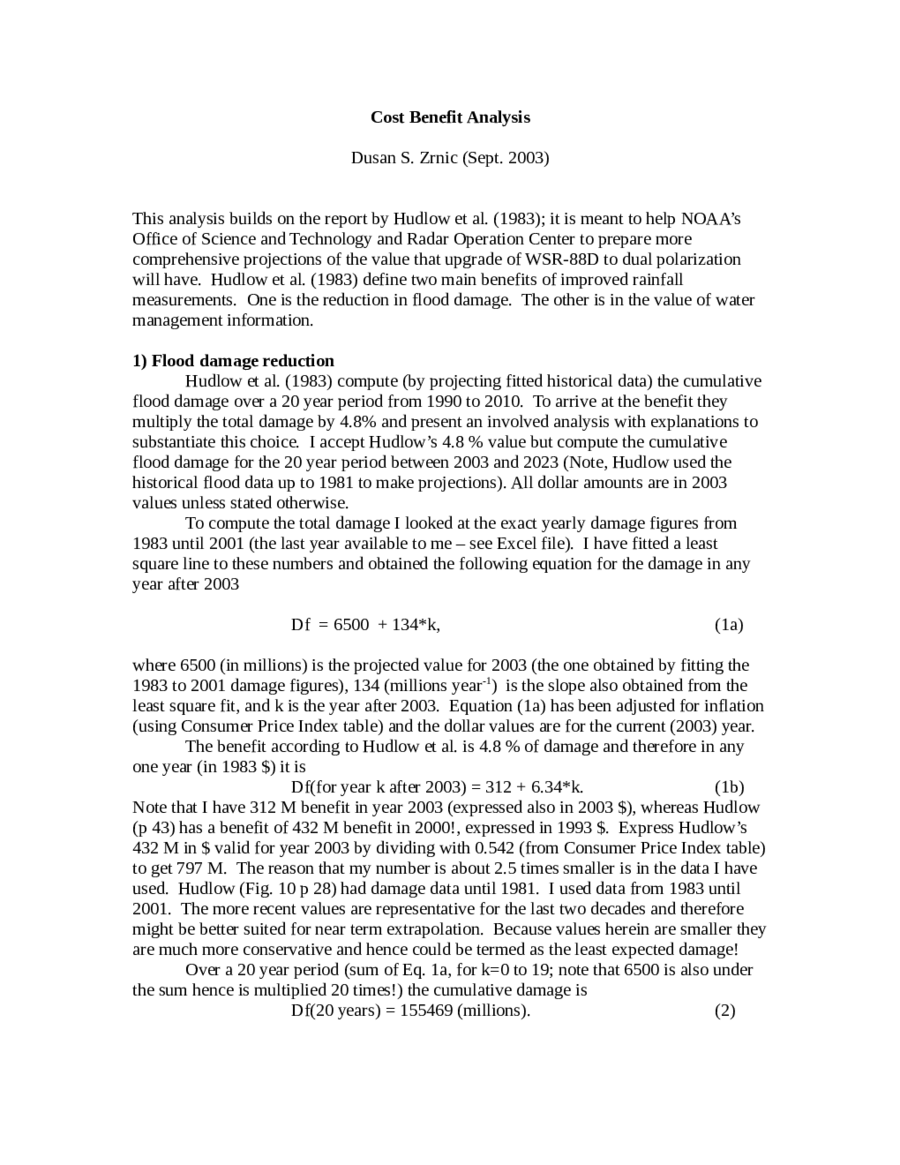
The benefits computed so far are for very good estimates of rainfall (where the
major uncertainty is few percent (see the attached figure after Hudlow et al. Fig 9). I
have modified the figure to be valid for the 2003 estimate of benefits explained in the
previous two sections. This modified figure (Fig. 1 herein) requires further explanation.
First the point on the ordinate at zero benefit is 1701+312 = 2013 M$ (from eqs.
1a and 4) and corresponds to the 729 M$ on the Hudlow graph. Then the other two break
points were proportionally increased by the ratio 2013/729 = 276; that is how I got 1676
M at about 24% reduction in accuracy and 276 at about 42 % accuracy reduction. (Note
276 corresponds to the 100 M on Hudlow’s graph, and I read the break points with the
help of ruler).
My label “Benefits from full implementation of the pre WSR-88D capability” is
at the level corresponding to Hudlow’s “Benefits from full implementation of current
radar capability”, again scaled by 276. Hudlow et al. refer to what the capability of the
radar prior to the WSR-88D would have been if these radars were modernized without
change in specifications. Accelerated loss in benefits from increasing error in inputs and
runoff model magnification is also where Hudlow et al. have put it (with changes due to
inflation and my computation in the previous section). I have added two more benefit
thresholds. One is “Current Benefits (2003)” and the other is “Benefits from full
implementation of polarimetric capability”. This is where the angels are, and you find
them!; my earnest try is in the following paragraph.
I have equated the current percent reduction in accuracy with the accuracy I
believe is achieved with the current system in operation (as is today! Please ROC – NWS
check this number – do you agree if not pick an accepted number %). It seems that
rainfall estimated from the reflectivity factor has an overall 30 % reduction in accuracy of
what might be ideally possible. This number is quoted by Balakrishnan et al. (1989) as
the average absolute deviation (AAD) between disdrometer measurement and computed
rain rates from disdrometer data via a synthetic R(Z) algorithm; it also follows from latest
report by Ryzhkov (2003). The report (Fig 10 in Ryzhkov 2003) shows that a 4 times
reduction in RMS error (i.e., RMS difference between radar and rain gauges) over an area
is expected with polarimetric rainfall estimator compared to the R(Z) estimate. For point
measurements the RMS difference between gauges and radar is about 2 times smaller for
the polarimetric estimator.
Now, let’s see how to translate the RMS errors that Ryzhkov expresses in mm into
% error in Fig 1. Polarimetric aficionados would tell you that they expect under ideal
conditions to have about 10 % error with a good polarimetric estimator (10 to 15% is the
AAD quoted by Balakrishnan et al. 1989, their table 2). If we accept this then the
reflectivity estimate from Ryzhkov’s paper would be at a 40% level (four times larger) for
area rainfall measurements. But for best point measurements we would have larger errors
in both polarimetric and R(Z). If we accept point polarimetric measurement to be at 15%
level than we would have a 30 % level for R(Z).
Overall I think that the polarimetric method could achieve 10 % accuracy. Thus,
the difference between achievable (1870) and current (1144) is a conservative estimate of
the potential benefit (726 million) if polarimetry were to be implemented today (the year
2003). Note that choice of other points on the graph would make some non alarming
deviation from my result. That is, if there is an offset in both points the difference
between the two points will change little; if anything we expect the offsets to be negative
which would make the benefits larger. Perhaps a range of values to the percent of
reduction corresponding to R(Z) and polarimetric method should be assigned?
Next cumulative benefits that are achievable over the 20 year span starting with
2003 are computed following the reasoning in this discussion.
Thus achievable cumulative benefit from flood damage reduction with full polarimetric
capability becomes:
Bfp = Bf(20 years)*1870/2013 = 6932, (6)
and the achievable benefit from better water management is
Bwmp = Bwm(20 years)* 1870/2013 = 39016. (7)
Current cumulative benefit from flood damage reduction – on the WSR-88D network
Bfc = Bf(20 years)*1144/2013 = 4241. (8)
Current cumulative benefit from better water management
Bwmc = Bwm(20 years)*1144/2013 = 23869. (9)
Therefore the total projected benefit over 20 years (starting with 2003 ending in 2023)
equals Eq(6)-Eq(8)+Eq(7)-Eq(9) = 17838 millions in dollar values of the current year
(2003).
0 10 20 30 40 50 60 70 80 90 100
0
276
552
828
1104
1380
1656
1932
2208
Percent reduction in accuracy
Hydrologic benefits (in million $)
Benefits from full implementation of
pre WSR-88D capability
Current Benefits (2003)
Accelerated loss in benefits from increasing error
in inputs and runoff model magnification
Benefits from full implementation of polarimetric capability
1870
1144
414
Fig 1. Possible benefits vs percent reduction in accuracy (adapted from Hudlow et al.
1983) for year 2003 expressed in current (2003) value of dollar.
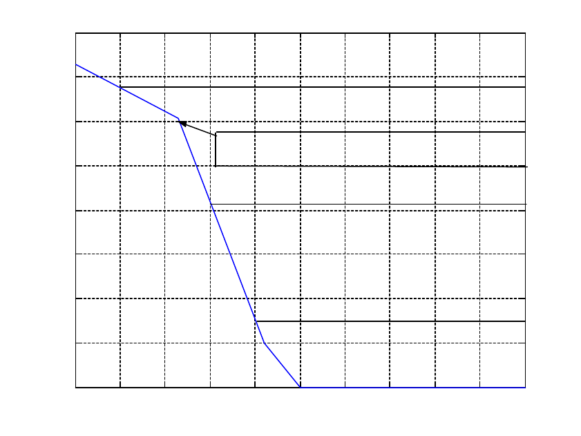
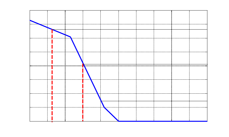
A graph of benefits for a slightly larger errors in polarimetric rainfall estimates
(12 % compared to 10 %) is presented in the appended figure.
Possibly a more realistic cost effectiveness would be to express the benefits
starting with the year 2008 (when dual polarization capability should become available).
This is easy to do by following the procedure established herein. A further consideration
is the lifetime of the polarimetric network. Will it be 20 years from 2008?
References
Blakrishnan, N., D.S. Zrnic, J. Goldhirsh, and J. Rowland, 1989: Comparison of
simulated rain rates from disdrometer data employing polarimetric radar algorithms. J.
Atmos. Oceanic. Tech. 6, 476-486.
Hudlow M.D., R.K. Farnsworth, and P.R. Anhert, 1983: NEXRAD technical
requirements for precipitation estimation and accompanying economic benefits. Hydro
Technical Note – 4. Office of Hydrology, National Weather Service, NOAA, p 49.
Ryzhkov, V.R, 2003: Rainfall measurement with a polarimetric WSR-88D. NSSL report
prepared to the Office of System Technology and Office of Hydrology, p 100+.
Consumer Price Index (CPI) Conversion Factors 1800 to estimated 2013 to Convert to
Dollars of 2003(estimated).
0 10 20 30 40 50 60 70 80 90 100
0
276
552
828
1104
1380
1656
1932
2208
Accuracy in rainfall measurement (%)
Hydrologic benefits (in million $)
Benefits from full implementation
of pre WSR-88D capability
Benefits (2003)
Benefits from full implementation of pol capability
1834
1144
414
Fig. 1 Alternate – from power point presentation – with a slightly relaxed 12% achievable
accuracy.
Yours truly, Dusan Zrnic – Graduate Research Assistant to the Harmonious one
and in service of the Wise One.