Fillable Printable Instruction Sheet for Amortization Schedule on Excel

Instruction Sheet for Amortization Schedule on Excel

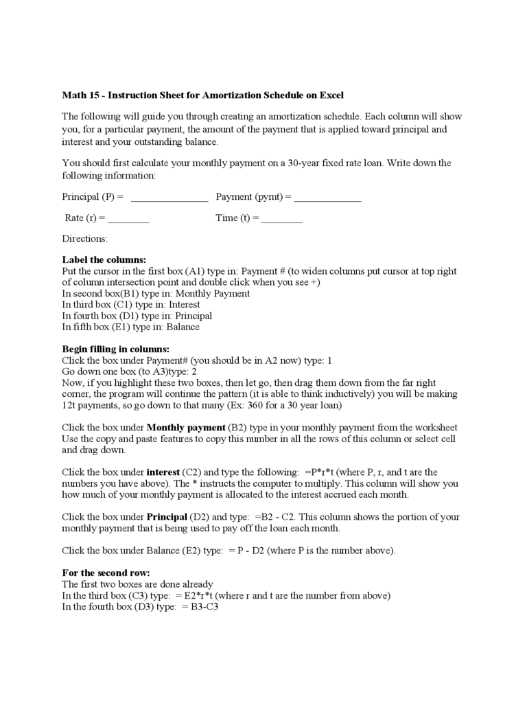
Math 15 - Instruction Sheet for Amortization Schedule on Excel

The following will guide you through creating an amortization schedule. Each column will show

you, for a particular payment, the amount of the payment that is applied toward principal and

interest and your outstanding balance.

You should first calculate your monthly payment on a 30-year fixed rate loan. Write down the

following information:

Principal (P) = _______________ Payment (pymt) = _____________

Rate (r) = ________ Time (t) = ________

Directions:

Label the columns:

Put the cursor in the first box (A1) type in: Payment # (to widen columns put cursor at top right

of column intersection point and double click when you see +)

In second box(B1) type in: Monthly Payment

In third box (C1) type in: Interest

In fourth box (D1) type in: Principal

In fifth box (E1) type in: Balance

Begin filling in columns:

Click the box under Payment# (you should be in A2 now) type: 1

Go down one box (to A3)type: 2

Now, if you highlight these two boxes, then let go, then drag them down from the far right

corner, the program will continue the pattern (it is able to think inductively) you will be making

12t payments, so go down to that many (Ex: 360 for a 30 year loan)

Click the box under Monthly payment (B2) type in your monthly payment from the worksheet

Use the copy and paste features to copy this number in all the rows of this column or select cell

and drag down.

Click the box under interest (C2) and type the following: =P*r*t (where P, r, and t are the

numbers you have above). The * instructs the computer to multiply. This column will show you

how much of your monthly payment is allocated to the interest accrued each month.

Click the box under Principal (D2) and type: =B2 - C2. This column shows the portion of your

monthly payment that is being used to pay off the loan each month.

Click the box under Balance (E2) type: = P - D2 (where P is the number above).

For the second row:

The first two boxes are done already

In the third box (C3) type: = E2*r*t (where r and t are the number from above)

In the fourth box (D3) type: = B3-C3

In the fifth box (E3) type: = E2 - D3

Now, you don't want to be doing this 360 times. So the program will do the rest for you:

Highlight the 3 boxes you just did (C3,D3,E3), let go, then drag the far right corner down to the

bottom of your spread sheet. Your balance should be 0 (it may not be exactly zero but could be a

small number due to round off error).

Below the last row, in the first column, type: totals:

In the C column type in: = sum(C2:Ck)where k is the column number of the last payment cell

(this will add all the numbers in this column starting with C2 through Ck)

Do the same in the D column - type: =sum(D2:Dk) this should add up to a number that is very

close to your loan amount

Graphs:

You can use the Excel program to make the following graphs.

For each year of your loan (every 12 payments) find the interest amount and plot it as the y-value

with the year number as the x-value. On the same axes, plot the principal amount versus year

(use a different color). Indicate where the two graphs cross and discuss what happens after this

point.

Questions:

1. What happens to the interest as you go down this column?

2. What happens to the amount allocated to principal as you go down that column?

3. After how many months was the balance of the loan half of the original amount? (The answer

will not be half-way through the loan period)